ArcGIS Online – Master of Spatial Analysis

Spatial Intelligence Dashboard for Community Safety Using ArcGIS for Power BI

Geovis Project Assignment, TMU Geography, SA8905, Fall 2025

By Debbie Verduga

Welcome to my Geo Viz Tutorial!

I love ArcGIS and I love Power BI. Each shines in their own way, which is why I was excited to discover the new ArcGIS integration within Microsoft Power BI. Let’s dive in and explore what it can do!

First off, traditional business intelligence (BI) technologies offer powerful analytical insights but often fall short in providing geospatial context. Conversely, geospatial technologies offer map centric capabilities and advanced geoprocessing, but often lack insights integration.

ArcGIS for Power BI directly integrates spatial analytics with business intelligence without the need of geoprocessing tools or advanced level expertise. This integration has the potential to empower everyday analysts to explore and leverage spatial data without needing to be highly experts in GIS.

This tutorial will demonstrate how to use ArcGIS for Power BI to:

Integrate multiple data sources – using City of Toronto neighbourhood socio-demographics, crime statistics, and gun violence data.
Perform data joins within Power BI – by linking datasets effortlessly without needing complex GIS tools.
Create interactive spatial dashboards – by blending BI insights with mapping capabilities, including thematic maps and hotspot analysis.

You will need TMU Credentials for:

Power BI Online
ArcGIS Online
Data

Dataset	File Type	Source
Neighbourhood Socio-demographic Data	Excel	Simply Analytics (Pre-Aggregated Census Data)
Neighbourhood Crime Rates	SHP File (Boundary)	ArcGIS Online Published by Toronto Police Service
Shooting & Firearm Discharge	SHP File (Point/Location)	ArcGIS Online Published by Toronto Police Service

Power BI Online

Log into https://app.powerbi.com/ using your TMU credentials. To help you out, watch this tutorial to get started with Power BI Online.

ArcGIS Online

Log Into https://www.arcgis.com/ using your TMU credentials. Make sure you explore data available for your analysis. For this tutorial we will be using Toronto Police Service Open data including neighbourhood crime rates and shootings and firearms discharges.

Loading Data

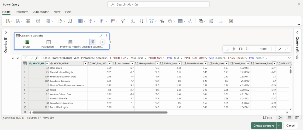
To create a new report in Power BI, you need a set of data to start. For this analysis, we will use neighbourhood level socio-demographic data in an excel format. This data includes total population and variables that are often associated with marginalized communities including low income, unemployment rates, no education and visible minorities rates. This data does not have spatial reference, however, the neighbourhood name and unique identifier is available in the data.

Add Data > Click on New Report > Get Data > Choose Data Source > Upload File > Browse to your file location > Click Next > Select Excel Tab you wish to Import > Select Transform Data

Semantic Model

This will take you to the report’s Semantic Model. Think of a semantic model as the way you transform raw data into a business-ready format for analysis and reporting. The opportunities for manipulating data here are endless!

Using the semantic model you can define relationships with other data, incorporate business logic, perform calculations, summarize, pivot and manipulate data in many ways.

What I love about semantic models is that it remembers every transformation you have made to the data. If you made a mistake, don’t sweat it, come back to the semantic model and undo. It’s that simple.

Once you load data you have two options. You can create a report or create a semantic model. Let’s create a report for now.

Create Report > Name Semantic Model

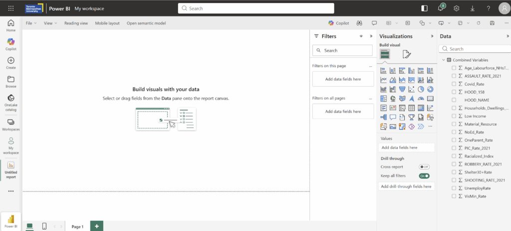
Report Layout

The report layout functions as a canvas. This is where you add all your visualizations. On the right panel you have Filters, Visualizations and Data.

Visuals are added by clicking on the icons. If you hover over the icon, you can see what they are called. There are default visuals, but you can add more visuals from the microsoft store.

The section below the visual icons helps guide how to populate the visual with your data.

Each visual is configured differently. For example, a chart/graph requires a y-axis and y-axis. To populate these visuals, drag and drop the column from your data table into these fields/values.

Add a Visual

Lets add an interactive visualization that displays the low income rate based on the neighbourhood selected from a list.

From the visualization panel > Add the Card Visual

From the data panel > Drag the variable column into the Fields

By default, Power BI summarizes the statistics in your entire data. Lets create an interactive filter to interact with this statistic based on a selected neighborhood.

From the Visualizations Panel > Add the Slicer Visual > Drag and drop the column that has the neighbourhood name > Filter from the slicer any given neighbourhood.

The slicer now interacts with the Card visual to filter out its respective statistic.

Congrats! We have created our very first interactive visualization! Well done :)

Pro Tip: To validate that calculations and visualizations are correct in Power BI, use excel to manipulate data in the same format and validate that visualizations are correct.

Load Data from ArcGIS Online

To demonstrate the full integration of Power BI and geospatial data, let’s bring data from ESRI’s ArcGIS Online. Authoritative open data is available in this portal and can be directly accessed through Power BI.

Linking Data

When you think about integrating non-spatial data with spatial/location data, you will need to keep in mind that at the very least, you will need common identifiers to be able to link data together. For example, the neighbourhood data has a neighbourhood name and identifier which are also available in the data published by the Toronto Police Service including neighbourhood crime rates and shootings and firearms discharges.

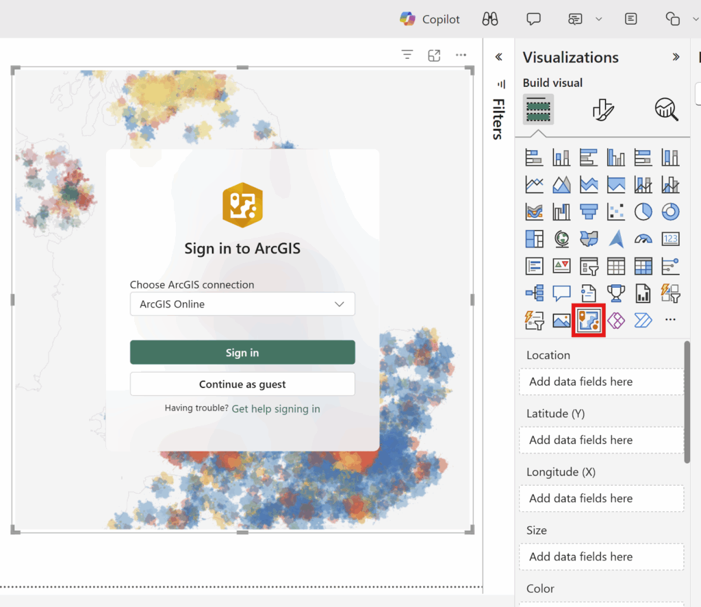
Add ArcGIS for Power BI Visual

Add the ArcGIS for Power BI visual > Log in using your TMU Credentials.

Add Layers

Click on Layers Icon > Switch to ArcGIS Online > Search for Layers by Name > Select Layer > Done

This will add the layer to your map. You can go back and add more layers. You can also add layers from your own ArcGIS Online account.

ArcGIS Navigation Menu

The navigation menu on the left panel of this window allows you to perform the following geospatial functions

Change and style symbology
Change the Base Map
Change Layer Properties
Analysis tab allows you to
- Conduct Drive Time and Buffer
- Add demographic data
- Link/Join Data
- Find Similar Data

For the purposes of this analysis, we will:

Establish a join between our neighbourhood socio-demographic data and the spatial data including crime rates and shootings and firearms discharges
Develop a thematic map of one crime type
Develop a shootings hot spot analysis

Data Cleansing

When linking data, the common neighbourhood IDs from all these different data sources are not in the same format. For example, in my data, the ID is an integer format. However, in the Shooting and Firearms Data, this field is in a text format padded with zeros.

In Power BI, we can create a clean table with neighbourhood information that acts as a neighbourhood dimension table to link data together and manipulate the columns to facilitate data linkages. Let’s create a neighbourhood dimension table.

Create a clean Neighbourhood Table

Open the Semantic Model > Change to Editing Mode > Transform Data > Right Click on Table > Duplicate Neighbourhood Table > Right Click on new table to Rename > Choose Column > Remove all Unwanted Columns > Click on Hood ID Column > Click Transform > Change to Whole Number > Right Click on Column to Rename > Add Custom Column (Formula Below) > Save

Formula = Text.PadStart(Text.From([HOOD_158]), 3, “0”)

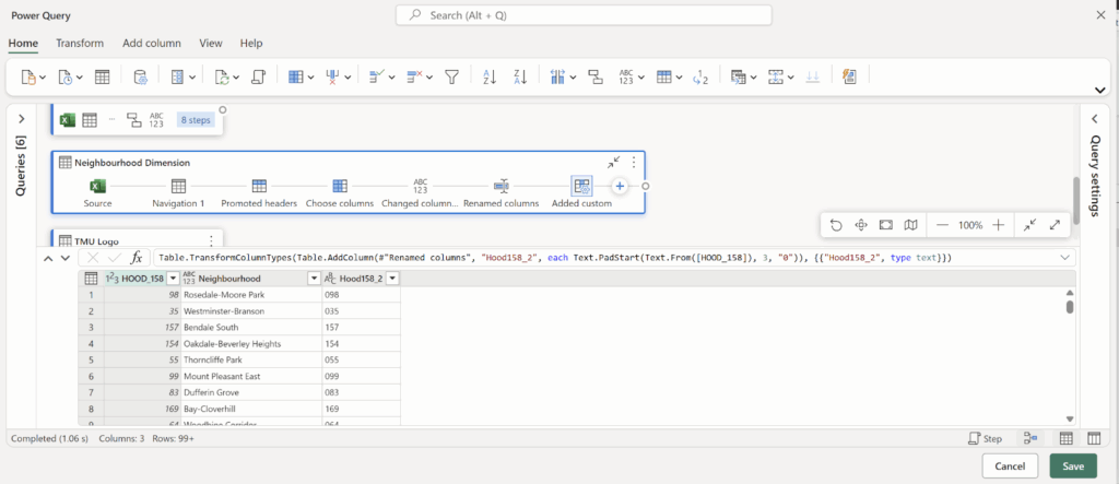
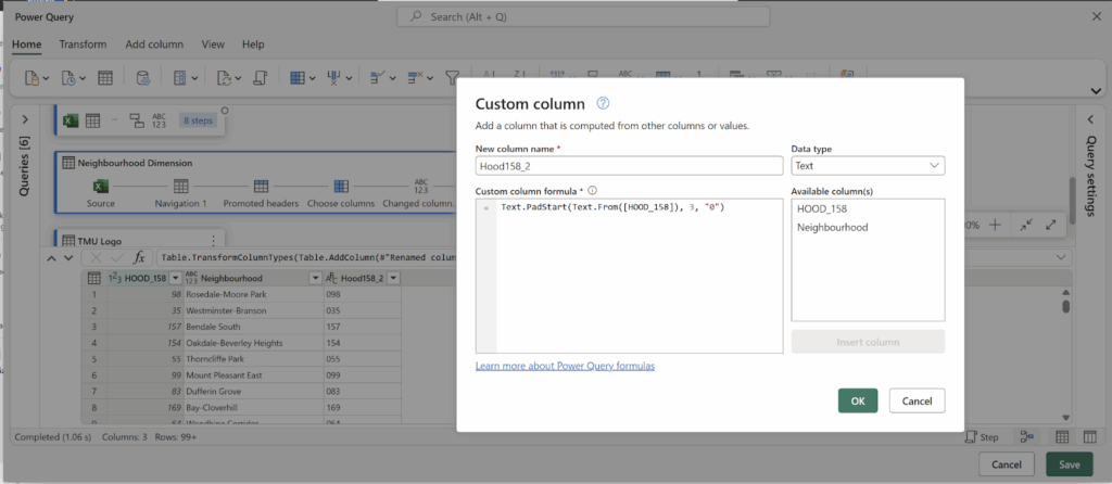
The custom column and formula takes the HOOD ID, changes it into a text field and adds padding of zeros. This will match the neighbourhood ID format in the shootings and firearm discharge data. Keep in mind, the only data you can manipulate is the data within your semantic model. You cannot change or manipulate the data sourced from ArcGIS Online.

Relationships

The newly created table in the semantic model needs to be related to the neighbourhood socio-demographic data to make sure that all tables are related to each other.

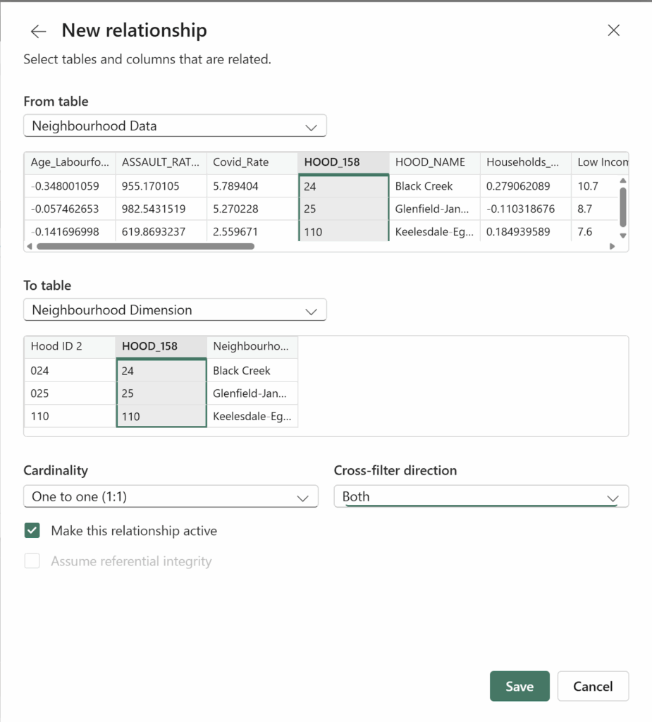
Establish a Relationship

In the semantic model view > Click Manage Relationships > Add New Relationship > Select From Table and Identifier > Select To Table and Identifier > Establish Cardinality and Cross-Filter Direction to Both > Save > Close

Congrats! We created a clean table that will function as a neighbourhood dimension table to facilitate data joins. We also learned how to establish a relationship with other tables in your semantic model. This comes handy as you can integrate multiple sources of data.

Let’s return to the report and continue building visualizations.

Joining Non-Spatial Data with Spatial Data

Neighbourhood Crime

Now we will join our non-spatial data from our semantic model with our spatial data in ArcGIS Online.

Join Non-Spatial Data with ArcGIS Online Data

Click on the ArcGIS Visual > Analysis Tab > Join Layer > Target Layer > Power BI Data (Drag & Drop Hood ID into the Join Layer Field in the Visualization Pane > Additional Options will now Appear on the Map> Select Join Field > Join Operation Aggregate > Interaction Filter > Create Join > Close

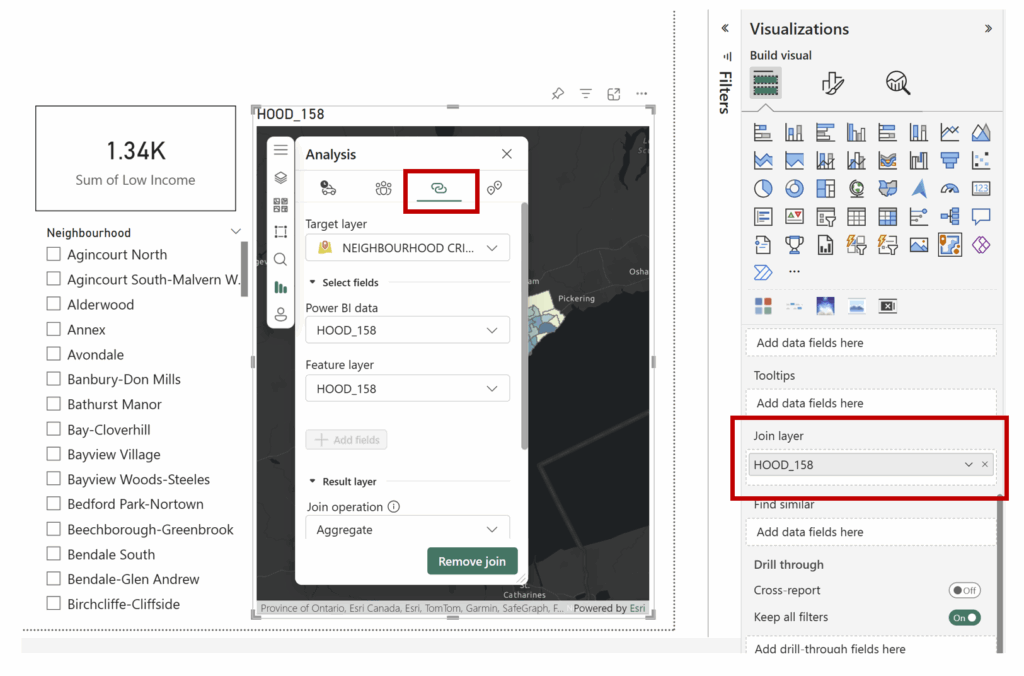
Congrats! We have created a join between the non-spatial data in Power BI and the spatial data in ArcGIS Online.

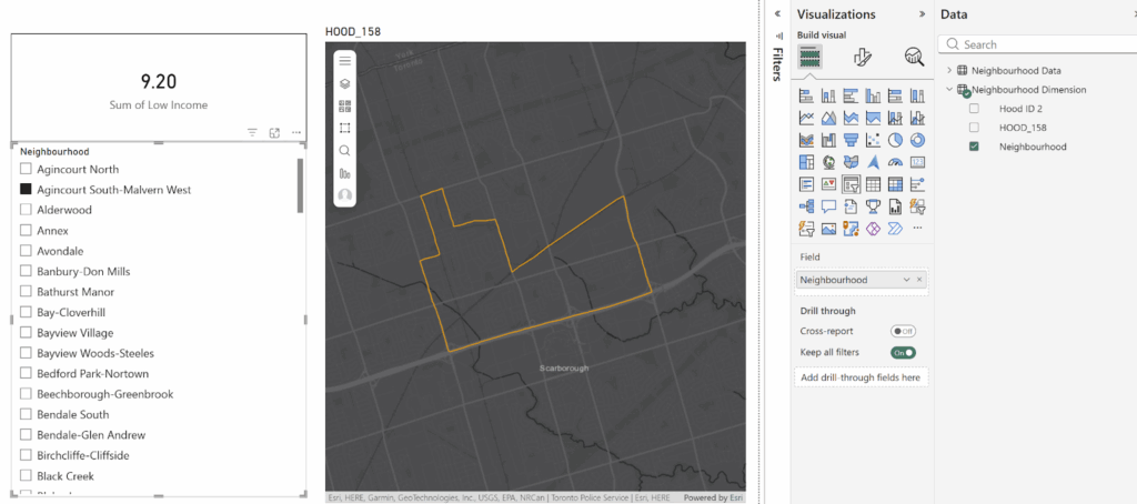
Change the neighbourhood filter to see this map filter and zoom into the selected neighbourhood.

Thematic Map

Now, let’s create a thematic map with one of the crime rates variables in this dataset.

On the left hand panel of the map:

Click on Layers > Click on Symbology > Active Layer > Select Field Assault Rate 2024 > Change to Colour > Click on Style Options Tab > Change Colour Ramp to another Colour > Change Classification > Close Window.

Congrats! We created a thematic map in Power BI using ArcGIS Online boundary file.

Change the neighbourhood filter to see how the map interacts with the data. Since this is a thematic map, we may not want to filter all the data, instead, we just want to highlight the area of interest.

Click on Analysis > Join Layer > Change the Interaction Behaviour to Highlight instead of Filter> Update Join

Check this again by changing the neighbourhood filter. Now, the map just highlights the neighbourhood instead of filtering it.

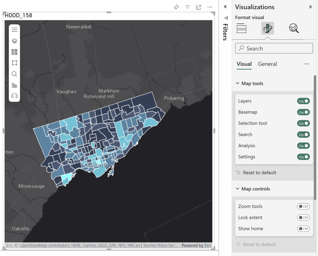
Customizing Map Controls

When you have the ArcGIS visual selected, you have the ability to customize your settings using the visualization panel. This controls the map tools available in the report. This can come in handy when setting up a default extent in your map for this report or allowing users to have control over the map.

Shootings and Firearm Discharges

Let’s visualize location data and create a hot spot analysis. To save time, copy and paste the map you created in the step before.

In the new map, add the Shootings and Firearms Data.

Challenge: Practice what you have learned thus far!

Change the base layer to a dark theme.
Add the Shootings and Firearm Discharge Data from ArcGIS Online.
Create a join with this layer and the data in Power BI.
Play around with changing the colour and shape of the symbology.

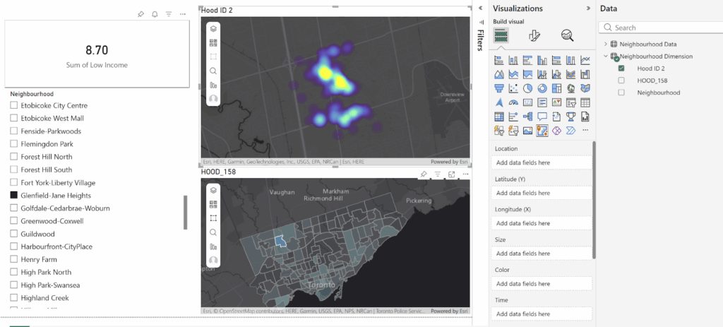
Hotspot Analysis

Now create a heat map from the Shooting and Firearm Discharges location data.

Click on Layers > Symbology > Change Symbol Type from Location to Heat Map > Style Options > Change Colour Ramp > Change Blur Radius > Close

Congrats! We have created a heat map in Power BI!

This map is dynamic, when you filter the neighbourhood from the list, the hot spot map filters as well.

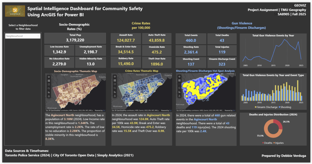
Customizing your report

It’s time to customize the rest of the report by adding visualizations, incorporating additional maps, adjusting titles and text, changing the canvas background, and bringing in more data to enrich the overall analysis.

I hope you’re just as excited as I am to start using Power BI alongside ArcGIS. By blending these two powerful tools, you can easily bring different data sources together and unlock a blend of BI insights and spatial intelligence—all in one place.

References

Neighbourhood Crime Rates – Toronto Police Service Open Data

Shooting and Firearm Discharges – Toronto Police Service Open Data

Environics Analytics – Simply Analytics

Evolution of Residential Real Estate in Toronto – 2014 to 2022

Shashank Prabhu, Geovis Project Assignment, TMU Geography, SA8905, Fall 2024

Introduction
Toronto’s residential real estate market has experienced one of the most rapid price increases among major global cities. This surge has led to a significant affordability crisis, impacting the quality of life for residents. My goal with this project was to explore the key factors behind this rapid increase, while also analyzing the monetary and fiscal policies implemented to address housing affordability.

The Approach: Mapping Median House Prices
To ensure a more accurate depiction of the market, I used the median house price rather than the average. The median better accounts for outliers and provides a clearer view of housing trends. This analysis focused on all home types (detached, semi-detached, townhouses, and condos) between 2014 and 2022.

Although data for all years were analyzed, only pivotal years (2014, 2017, 2020, and 2022) were mapped to emphasize the factors driving significant changes during the period.

Data Source
The Toronto Regional Real Estate Board (TRREB) was the primary data source, offering comprehensive market watch reports. These reports provided median price data for Central Toronto, East Toronto, and West Toronto—TRREB’s three primary regions. These regions are distinct from the municipal wards used by the city.

Creating the Maps

Step 1: Data Preparation
The Year-to-Date (YTD) December figures were used to capture an accurate snapshot of annual performance. The median price data for each of the years across the different regions was organized in an Excel sheet, joined with TRREB’s boundary file (obtained through consultation with the Library’s GIS department), and imported into ArcGIS Pro. WGS 1984 Web Mercator projection was used for the maps.

Step 2: Visualization with 3D Extrusions
3D extrusions were used to represent price increases, with the height of each bar corresponding to the median price. A green gradient was selected for visual clarity, symbolizing growth and price.

Step 3: Overcoming Challenges

After creating the 3D extrusion maps for the respective years (2014, 2017, 2020, 2022), the next step was to export those maps to ArcOnline and then to Story Maps, the easiest way of doing so was to export it as a Web Scene, from which it would show up under the Content section on ArcOnline.

Flattened 3D Shapes: Exporting directly as a Web Scene to add onto Story Maps caused extrusions to lose their 3D properties. This was resolved using the “Layer 3D to Feature Class” tool.

Lost Legends: However, after using the aforementioned tool, the Legends were erased during export. To address this, static images of the legends were added below each map in Story Maps.

Step 4: Finalizing the Story Map
After resolving these issues, the maps were successfully exported using the Export Web Scene option. They were then embedded into Story Maps alongside text to provide context and analysis for each year.

Key Insights
The project explored housing market dynamics primarily through an economic lens.

Interest Rates: The Bank of Canada’s overnight lending rate played a pivotal role, with historic lows (0.25%) during the COVID-19 pandemic fueling a housing boom, and sharp increases (up to 5% by 2023) leading to market cooling.
Immigration: Record-breaking immigration inflows also contributed to increased demand, exacerbating the affordability crisis.

While earlier periods like 2008 were critical in shaping the market, boundary changes in TRREB’s data made them difficult to include.

Conclusion
Analyzing real estate trends over nearly a decade and visualizing them through 3D extrusions offers a profound insight into the rapid rise of residential real estate prices in Toronto. This approach underscores the magnitude of the housing surge and highlights how policy measures, while impactful, have not fully addressed the affordability crisis.

The persistent rise in prices, even amidst various interventions, emphasizes the critical need for increased housing supply. Initiatives aimed at boosting the number of housing units in the city remain essential to alleviate the pressures of affordability and meet the demands of a growing population.

Link to Story Map (You will need to sign in through your TMU account to view it): https://arcg.is/WCSXG

Mapping Child Friendly City Initiatives in Canada and in the World using ArcGIS StoryMaps

Anastasiia Smirnova
SA8905 Geovis project, Fall 2022

Introduction

Through this project I wanted to gain and advance my skills in both storytelling and visualizing spatial data. Here you can learn more about my attempt of using ArcGIS StoryMaps to highlight the importance of including children in the urban planning agenda and to show the World- and Canada-wide spatial patterns of urban areas’ commitment to creating inclusive urban environments with children in mind.

I did it by mapping municipalities that are participating in UNICEF’s Child Friendly Cities Initiatives (CFCI), which aim to promote cities where the “ voices, needs, priorities and rights of children are an integral part of public policies, programs and decisions.”

Technology

I used ESRI’s ArcGIS Pro, Online Map Viewer and StoryMaps for my project. First, I used the desktop app (ArcGIS Pro) to import my data and create my initial maps. After that I uploaded the layers that I wanted to use as web layers to my ArcGIS account, and then I finalized them using ArcGIS online applications. I used the online map viewer to adjust symbology as necessary as was trying to figure out what worked better for each part of my story. It was easy to go back and forth between the Map Viewer and StoryMaps – to make the necessary changes, then to see how the updated maps work with the story, and then repeat these steps as needed. The Map viewer generally had the functionality I needed to change my map symbology and I did not have to go back to ArcGIS Pro too often to make modifications after I uploaded my layers online.

I liked the functionality of StoryMaps. I used the sidecar option to introduce my story, and for showing most of my maps. I find that this block type provides some of the most immersive experience while scrolling, so I used it for the parts of the story that I wanted to keep the reader’s attention on.

I found that the swipe option worked well for showing comparisons. In a regular map, it is often difficult to show all information you want without cluttering the map with too many layers and making the map unreadable. The swipe option can help solve this problem. As such, I used this function to show how many children did (not) live within the municipalities that were part of CFCI and therefore could (not) benefit from the initiative.

the map shows distribution of children and youth residences (on the left, yellow and red) and municipalities involved in CFCI (on the right, blue)

For inserting your maps to any blocks of StoryMaps, you can choose to either use your maps uploaded as images or insert the actual interactive online maps. While the image option has some benefits, such as more flexibility in styling the map and faster loading, the main benefit of inserting the actual online maps is interactivity. You can zoom in and out, search for a specific location, show/hide legend, learn more about each unit on the map and so on (as the creator of the story, you can edit and set restrictions of what readers can and cannot do with your online maps).

Since I wanted to keep my maps as simple visually as possible, I went with the second option. This way, if the reader wanted to learn more about my maps and the information they displayed, they could do so by using the interactive map functions.

Interesting findings

In addition to the main message of the project (the need to promote child friendly cities), the maps showed how the choice of data, scale and mapping methodology can influence the results and representation. On the CFCI website, the main map was showing all countries that were involved in the CFCI. The map did not consider how many municipalities in each country were actually involved in the initiatives.

The main map from the UNICEF CFCI website – CFCI countries

This way of displaying data may be misleading, since the level involvement of each country varied greatly. In some countries, most of the territory was part of CFCI, but some other countries only had a couple municipalities each with UNICEF’s child friendly initiatives.

For this story, in addition to the world CFCI country map similar to the one from the website, a proportional symbol map was created to show how many municipalities from each country were actually involved in the CFCI and I put these two maps in one sidecar block so that the reader could swipe back and forth to see how the distribution of CFCI changed with the change of the variable, and what the actual level of involvement if each country was.

A map from my StoryMap – Municipalities involved in CFCI

When zoomed in, even more information about the unevenness and clustering in the spatial distribution of the CFCI municipalities can be discovered.

The sidecar block (I used the float side by side option for my maps), and the smooth transitions it provided, worked well for showing the differences between the maps, as well as for zooming in into a smaller scale map.

Challenges

Some of the main challenges for me were associated with updating the maps if I wanted to change something. It took some time for me to figure out what could be done at which step of the process (with different apps) and how far back I had to go to modify something. As such I had trouble updating and modifying the legends for the maps.

Unfortunately, the options for adjusting the legends using the ArcStory editor or the online map viewer were limited. For instance, it was impossible to hide or edit the name of the column which contained data used in the map while using the online apps. Since I was creating my original layers in ArcGIS Pro, then uploading them as web layers, and then adjusting my maps further in the online map viewer, it was difficult to go back to change the original data in the end, just to modify one little line on the map legend. Only some parts of the legend could be modified using the online apps. So, one of the lessons I took from this experience is that you need to make sure all the column names are appropriate before making all the edits online if you are using a similar process as I did. It is also helpful to think about the legends right from the start.

Conclusion and results

In general, I am satisfied with the ArcGIS StoryMap platform. It was easy to use, and it did a good job of assisting me in creating a map-based story that looks clean and flows smoothly. I am planning on further exploring the StoryMap functionality in the future.

If you are interested in learning more about child friendly cities and seeing my StoryMap result, you can follow this link:

Canadian cities and towns for happy children (arcgis.com)

COVID-19 in Toronto: A Tale of Two Age Groups

By Meira Greenbaum

Geovis Project Assignment @RyersonGeo, SA8905, Fall 2020

Story Map Link

Introduction

The COVID-19 pandemic has affected every age group in Toronto, but not equally (breakdown here). As of November 2020, the 20-29 age group accounts for nearly 20% of cases, which is the highest proportion compared to the other groups. The 70+ age group accounts for 15.4% of all cases. During the first wave, seniors were affected the most, as there were outbreaks in long-term care homes across the city. By the end of summer and early fall, the probability of a second wave was certain, and it was clear that an increasing number of cases were attributed to younger people, specifically those 20-29 years old. Data from after October 6th was not available at the time this project began, but since then Toronto has seen another outbreak in long-term care homes and an increasing number of cases each week. This story map will investigate the spatial distribution and patterns of COVID-19 cases in the city’s neighbourhoods using ArcGIS Pro and Tableau. Based on the findings, specific neighbourhoods with high rates can be analyzed further.

Why these age groups?

Although other age groups have seen spikes during the pandemic, the trends of those cases have been more even. Both the 20-29 and 70+ groups have seen significant increases and decreases between February and November. Seniors are more likely to develop extreme symptoms from COVID-19, which is why it is important to focus on identifying neighbourhoods with higher rates of seniors. 20-29 is an important age group to track because increases within that group are more unique to the second wave and there is a clear cluster of neighbourhoods with high rates.

Data and Methods

The COVID-19 data for Toronto was provided by the Geo-Health Research Group. Each sheet within the Excel file contained a different age group and the number of cases each neighbourhood had per week from January to early October. The format of the data had to be arranged differently for Tableau and ArcGIS Pro. I was able to table join the original excel sheet with the columns I needed (rates during the week of April 14th and October 6th for the specific age groups) to a Toronto neighbourhood shapefile in Pro and map the rates. The maps were then exported as individual web layers to ArcGIS Online, where the pop-ups were formatted. After this was done, the maps were added to the Story Map. This was a simple process because I was still working within the ArcGIS suite so the maps could be transported from Pro to Online seamlessly.

For animations with a time and date component, Tableau requires the data to be vertical (i.e. had to be transposed). This is an example of what the transformation looks like (not the actual values):

A time placeholder was added beside the date (T00:00:00Z) and the excel file was imported into Tableau. The TotalRated variable was numeric, and put in the “Columns” section. Neighbourhoods was a string column and dragged to the “Colour” and “Label” boxes so the names of each neighbourhood would show while playing the animation. The row column was more complicated because it required the calculated field as follows:

TotalRatedRanking is the new calculation name. This produced a new numeric variable which was placed in the “Rows” box.

If TotalRatedRanking is right clicked, various options will pop-up. To ensure the animation was formatted correctly, the “Discrete” option had to be chosen as well as “Compute Using —> Neighbourhoods.” The data looked like the screenshot below, with an option to play the animation in the bottom right corner. This process was repeated for the other two animations.

Unfortunately, this workbook could not be imported directly into Tableau Public (where there would be a link to embed in the Story Map) because I was using the full version of Tableau. To work around this issue, I had to re-create the visualization in Tableau Public (does not support animation), and then I could add the animation separately when the workbook was uploaded to my Tableau Public account. These animations had to be embedded into the Story Map, which does have an “Embed” option for external links. To do this, the “Share” button on Tableau Public had to be clicked and a link appeared. But when embedded in the Story Map, the animation is not shown because the link is not formatted correctly. To fix this, the link had to be altered manually (a quick Google search helped me solve it):

Limitations and Future Work

Creating an animation showing the rate of cases over time in each neighbourhood (for whichever age group or other category in the excel spreadsheet) may have been beneficial. An animation in ArcGIS Pro would have been cool (just not enough time to learn about how ArcGIS animation works), and this is an avenue that could be explored further. The compromise was to focus on certain age groups, although patterns between the start (April) and end (October) points are less obvious. It would also be interesting to explore other variables in the spreadsheet, such as community spread and hospitalizations per neighbourhood. I tried using kepler.gl, which is a powerful data visualization tool developed by Uber, to create an animation from January to October for all cases, and this worked for the most part (video at the end of the Story Map). The neighbourhoods were represented as dots (not polygons), which is not very intuitive for the viewer because the shape of the neighbourhood cannot be seen. Polygons can be imported into kepler.gl but only as a geojson and I am unfamiliar with that file format.

Toronto’s Waterfront Parking Lot Transformation

Author Name: Vera Usherovich

StoryMap Project link: https://arcg.is/004vSb

SA 8905 Fall 2020

Introduction:

During one of my study breaks, I was looking at aerial photographs of Toronto’s Waterfront. One thing in particular caught my attention; the parking lots. I did not grow up in Toronto and had no idea how drastically different the waterfront area looked like. I kept on opening up images from various years and comparing the changes. The Waterfront area was different; at first the roundhouses disappeared and followed by parking lots and industrial warehouses. This is the short answer to what inspired this StoryMap. I wanted to see how the surface of our city changed over time, specifically the role of parking lots.

Key Findings

There has been a 32 % reduction in surfaces dedicated to parking lots between 2003 and 2019.
Even though there are fewer parking lots, there is a similar proportion of parking lot size surfaced between 2003-2019.
Many of the parking lots in the entertainment district turned into condos.

About the StoryMap

Data

For this project, I used areal photographs from the City of Toronto, works and Emergency Services. I chose 2003 and 2019 as my years to compare.

Platform and Method

The digitization process was done through Esri’s software, ArcMap. I then exported the layers into gis online and made a map. this map was embedded into the StoryMap with adjustment to the layers. Additionally, I cross-referenced information with google maps, to identify what has replaced the parking lots (broke into 4 categories: residential, commercial, public, and other).

Limitations

Note: The data showcased in this story and maps is based on manual aerial photograph digitization. Some features might have been inadvertently missed or incorrectly categorized.

Future Work

This can be done for a wider range of years. Also, a more comprehensive classification of what is no longer a parking lot could be described in greater detail.

Toronto Raptors 2019-2020 Atlas

Atlas Web App Link

Geovisualization Project, @RyersonGeo, SA8905, Fall 2020

By Nicolas Karwowski,

Background

Sports have always been a common ground that brings together people of different ethnic and cultural backgrounds. However, regardless of the sport at hand, issues of racism have always accompanied athletic competition. With the reignition of the Black Lives Matter movement in 2020, sports teams and their players had the chance to take a stand against racism in a bigger way than ever before. In my household, we’ve followed the Toronto Raptors basketball team for many years. With this following, we have come to learn the stories of not only our own team’s players but also those of their competitors. I can reliably say that I have spent many hours learning about the hardships and the achievements of athletes from across the globe. While I do not regret spending so much time learning about the diversity of this sport, I understand that others may not have this time. This is why I have chosen to create a geovisualization that represents the complexity of an athlete’s journey to the top and the diversity of my favourite televised sport.

Data

Thankfully most widely known athletes have easily available information about their journey to the NBA. This usually includes the place they were born, the various schools they attended to hone their skills, and the professional teams they may have played for before reaching the big league. While in-depth bios exist for each team’s core roster on NBA.com, Wikipedia gives concise summaries of player’s geographic movements throughout their lives. As seen on the right, these summaries can include the player’s date of birth, place of birth, the high schools they attended and their respective locations, the college(s) they attended as well as NBA and other professional teams they might have played on. This information would be vital in the creation of points summarizing the player’s journey to athletic stardom. The main limitation of this information source is that like with other Wikipedia pages, the information could be incorrectly added, sometimes with malicious intent. Lesser known players may also have missing information. Since some players had up to 10 different locations credited in their summaries, I chose to include only ten players from the Raptor’s championship-winning 2019-2020 roster. The mention of the roster’s season is of importance as players come and go as the years go on.

Methods

For each player in the visualization, I created a new point feature class in ArcGIS Pro. I entered the points in chronological order so that when I had to connect them later with arrows, the arrows would indicate their path from place to place. Due to the number of points, their accuracy was usually only tied to the listed city’s geographical location. With all the feature classes created, I then added a few new attribute columns so that points in the final visualization could include context.

These attributes included the name of the city, the name of the country the city was located in, the type of location with regards to the player’s life (Place of Birth, School, Professional Team, NBA Team) and the player associated with that point. With this completed, I could link each of the points within feature classes using the Points To Line tool in ArcGIS. The subsequent use of the Split Line at Vertice tools was then done so that arrows could be created between points and not just at the end of the line. Using the Feature Class to Shapefile tool, I was able to export all 20 of the shapefiles, half of which were points and the other half being lines, to ArcGIS Online.

While ArcGIS Online lacks much of the symbology customization available in the desktop version, I made do with a set of simple icons. A green circle would represent the player’s place of birth, schools would be shown as blue diamonds, orange squares symbolized professional basketball and purple stars depicted NBA teams. This type of symbology allows users to understand a player’s journey to the NBA including their ups and downs.

In the final geovisualization web app, users have the ability to customize the map to whatever level they would like. If a user wishes to see where all players are born, they have the ability to turn off all layers except for the Place Of Birth layer. Clicking on any of the remaining green circles creates a pop-up that gives details on what city is there, who is born there and when they were born (as seen above). Alternatively, any and all player layers can be hidden if a user would like to focus on a single-player (as seen below).

Future work

The project as it stands only encapsulates a minuscule sample of all athletes in the NBA. Ideally, this geovisualization would enable to not only view all the Toronto Raptors players but all the players that have ever played in the NBA. When envisioning the perfect visualization, I imagine a crowdsourced app that allows anybody to add their favourite players to the app. Unfortunately, this app is non-editable and many of the steps involved required non-user-friendly applications. This visualization is also deeply limited by ArcGIS Online’s lack of symbology and UI options. These limitations include but are not limited to a search option for the layers manager as well as a grouping option for the symbology tab. Additionally, it would be very interesting to add a timeline feature in the app which allows people to see how the world of basketball has changed over the last few decades in a geographical sense.

Geovisualization of the York Region 2018 Business Directory

(Established Businesses across Region of York from 1806 through 2018)

Project Weblink (ArcGIS Online): Click here or direct weblink at https://ryerson.maps.arcgis.com/apps/opsdashboard/index.html#/82473f5563f8443ca52048c040f84ac1

Geovisualization Project @RyersonGeo
SA8905- Cartography and Geovisualization, Fall 2020
Author: Sridhar Lam

Introduction:

York Region, Ontario as identified in Figure 1, with over one million people from a variety of cultural backgrounds is across 1,776 square kilometres stretching from Steeles Avenue in the south to Lake Simcoe and the Holland Marsh in the north. By 2031, projections indicate 1.5 million residents, 780,000 jobs, and 510,000 households. Over time, York Region attracted a broad spectrum of business activity and over 30,000 businesses.

Fig.1: Region of York showing context within Ontario, Greater Toronto Area (GTA) and its nine Municipalities.
(Image-Sources: https://www.fin.gov.on.ca/en/economy/demographics/projections/ , https://peelarchivesblog.com/about-peel/ and https://www.forestsontario.ca/en/program/emerald-ash-borer-advisory-services-program)

Objective:

To create a geovisualization dashboard for the public to navigate, locate and compare established Businesses across the nine Municipalities within the Region of York.

The dashboard is intended to help Economic Development market research divisions sort and visualize businesses’ nature, year of establishment (1806 through 2018), and identify clusters (hot-spots) at various scales.

Data-Sources & References:

Methodology:

First, the Business Directory updated as of 2018, and the municipal boundaries layer files, which are made available at the Open-Data Source of York Region, are downloaded. As shown in Figure 2, the raw data is analyzed to identify the Municipal data based on the address / municipal location distribution. It is identified that the City of Markham and the City of Vaughan have a major share.

Fig.2: The number of businesses and the percentage of share within the nine Municipalities of the York Region.

The raw-data is further analyzed, as shown in Figure 3, to identify the major business categories, and the chart below presents the top categories within the dataset.

Fig.3: Major Business Categories identified within the dataset.

Further, the raw data is analyzed, as shown in figure 4, to identify the businesses by the year of establishment, and identifies that most of the businesses within the dataset were established after the 1990s.

Fig 4: Business Establishment Years identified within the dataset.

The Business addressed data is checked for consistency, and Geocodio service is used to geocode the address list for all the business location addresses. The resulting dataset is imported into ArcGIS Map, as shown in figure 5, along with the municipal boundaries layers and checked for inconsistent data before being uploaded onto ArcGIS Online as hosted layers.

Fig.5: Business Locations identified after geocoding of the addresses across the York Region.

Once hosted on ArcGIS Online, a new dashboard titled: ‘Geovisualization of the York Region 2018 Business Directory’ is created. To the dashboard, the components are tested for visual hierarchy, and careful selection is made to use the following components to display the data:

Dashboard Title
Navigation (as shown in figure 6, is placed on the left of the interface, which provides information and user-control to navigate)
Pull-Down/ Slider Lists for the user to select and sort from the data
Maps – One map to display the point data and the other to display cluster groups
Serial Chart (List from the data)- To compare the selected data by the municipality
Map Legend, and
Embedded Content – A few images and videos to orient the context of the dashboard

The user is given a choice to select the data by:

Fig.6: User interface for the dashboard offering selection in dropdown and slider bar.

Thus a user of the dashboard can select or make choices using one or a combination of the following to display the results in on the right panes (Map, data-chart and cluster density map):

Municipality: By each or all Municipalities within York Region
Business Type: By each type or multiple selections
Business Establishment Year Time-Range using the slider (the Year 1806 through 2018)

For the end-user of this dashboard, results are also provided based on business locations identified after geocoding the addresses across the York Region, comparative and quantifiable by each of the nine municipalities shown in Figure 7.

Fig.7: Data-Chart displayed once the dashboard user makes a selection.

By plotting the point locations on a map, and simultaneously showing the clusters within the selected range (Region/ by Municipality / by Business Type / Year of Establishment selections), Figure 8.

Fig.8: Point data map and cluster map indicate the exact geolocation as well as the cluster for the selection made by the user across the York Region at different scales.

Results:

Overall, the dashboard provides an effective geovisualization with a spatial context and location detail of the York Region’s 2018 businesses. The business type index with an option to select one/ multiple at a time and the timeline slider bar offers an end-user of the dashboard to drill down to the information they seek to obtain from this dashboard. The dashboard design offers a dark theme interface maintaining a visual hierarchy of the different map elements such as the map title, legend, colour scheme, colour combinations ensuring contrast and balance, font face selection and size, background and map contrast, choice of hues, saturation, emphasis etc. The maps also offer the end-user to change the background map base layers to see the data in the context of their choice. As shown in figure 9 of location data and quantifiable data at different scales, the dashboard interface offers visuals to display the 30,000+ businesses across the York Region.

This image has an empty alt attribute; its file name is Capture-1-1024x496.jpg

Fig.9: Geovisualization Dashboard to display the York Region 2018 Business Directory across the Nine Municipalities of the York Region.

The weblink to access the ArcGIS Online Dashboard where it is hosted is: https://ryerson.maps.arcgis.com/apps/opsdashboard/index.html#/82473f5563f8443ca52048c040f84ac1

(Please note an ArcGIS Online account is required)

Limitation:

The 2018 business data across York Region contains over 38,000 data points, and the index/ legend of the business types may look cluttered while a selection is made as well. The fixed left navigation panel width is definitely a technical limitation because the pull-down display cannot be made wider. However, the legend screen could be maximized to read all the business categories clearly. There may be errors, incomplete or missing data in the compilation of business addresses. This dashboard can be updated quickly but requires a little effort, whenever there is an update of the York Region business directory’s new release in the coming years.

Mapping Toronto Flood Events by using Esri Operations Dashboard

Dashboard Web application: Toronto Flood Events 2013-2017

By: Mohamad Fawaz Al-Hajjar

Geovisualization Project, @RyersonGeo, SA8905, Fall 2019

Introduction:

Toronto has been affected by many flood events, but the biggest modern event happened in July, 8th, 2013, when a thunderstorm passed over the city and broke the record when Toronto received huge amount of rain reached to 126mm, that caused major transit delays, power outages, flight cancellations and many areas flooded throughout the city; in order to visualize such phenomena and monitor the number of events per Toronto ward, web application dashboard has been implemented to inactively visualize the historical data, which also could be used to map the real time data as an optimal way to utilize the web dashboards.

Geovisualization Methodology

The technology that has been used to interactively visualize flood events data in Toronto is Esri Operations Dashboard, which was released in December, 2017 and has become an effective tool for the Esri users, which allow them to publish their Web Maps via dashboard by applying simple configuration without writing a single line of code. The project has followed the below methodology.

Data Review and Manipulation

After obtaining the open data from two main sources, TRCA Open Data Portal and Toronto Open Data Portal, with other different data sources which have been reviewed and visualized in ArcMap application 10.7.1 release. Some of the data had to be cleansed, such as Flood Plain Mapping Index and property boundary shapefiles, other data were derived from polygon shapefile “flood-reporting-wgs84” for Toronto wards, where the total number of flood events stored by year from 2013-2017. A derived data-set produced as a point shapefile events points by using generating random point tool from polygon in ArcGIS ArcToolbox.

In addition, another data set have been created, the Property boundaries which have been intersected and clipped with the flood plain feature to generate the flooded properties per ward, which is also spatially joined with the wards to inherit its attributes. that could be configured in the dashboard to show the number of flooded properties per ward.

List of Data-Set Used:

Stormevents (derived from Flood reporting polygon) (Toronto open data)

Property per ward (derived from Property boundary and Flood reporting polygons) (Toronto open data)

Flood Events renamed to (Flood reporting polygons) (Toronto open data)

Toronto Shelters (Toronto open data)

GTA Watercourses (TRCA open data)

GTA Flood Plain (TRCA open data)

GTA Waterbodies (TRCA open data)

2. Data Publishing:

After getting the data ready, map produced in ArcMap where data symbolized then published to web map In ArcGIS Online, which will be the core map for the operation dashboard.

3. Creating the Dashboard:

In order to generate an Esri operation dashboard you need to be a member of ArcGIS Online organization, then have a published Web Map or hosted Feature Layer as an input to the dashboard.

Creating the dashboard went through many steps as described below:

Login to your ArcGIS Online organization using your username and password.
From the main interface click the App Launcher button as below snapshot

or you could also click on your Web Map application under Content in ArcGIS Online then click on Create Web App dropdown list to choose Using Operations Dashboard

Create Web App box will be opened to fill Title, Tag and Summary
The map will be opened into the dashboard, where you will start to add the widgets you need to your application from the drop-down menu as below snapshot.

Widgets will be added and configured as needed.

Toronto Flood Events Dashboard has included the most important widgets (Map, Header, Serial Chart, Pie Chart, Indicator, and List)

Once widget selected, the configuration box will be opened which is easy to be configured then will be dragged to be docked as needed

After adding multiple widgets, an important setting needs to be configured in the Map widget to set what is called an Action Framework, that happens when we change the map extent of the geographic area, then the other dashboard elements such as (Serial Chart, Pie Chart, Indicator, and List) will interactively be changed.

From the Map Widget go to Configure button, then select Map Actions tab, hit Add Action drop-down list then filter to choose other dashboard elements from the configuration box. the option When Map Extent Changes appears to let you filter and make action to other elements as well. Indeed, this is the most powerful tool in the dashboard.
Another configuration could be made in the Header element where you can insert a drop-down menu to map a certain feature by date, type, area or time, which is easily be configured in the dashboard web application.

After configuring all required elements, hit save then you can share or publish your dashboard web application with other users out of your organization.

To access the Dashboard click on the link below
Toronto Flood Events 2013-2017

Geovisualization Project Limitations:

The project was encountered two main limitations:

The data limitation:

Data limitations were taken most of the time to be defined, then after defining the available open data, many data cleansing and manipulation has been taking in terms of changing spatial reference to fit with online maps or changing the data format, which are still limited with the variables used, the derived events point generated randomly from the polygon shapefile “flood-reporting-wgs84” for Toronto wards to show the number of events per Toronto ward, which are not available as points from the main source; even though, the points still not accurate in location, but it give an idea about the number of event per ward boundary in different years.

Technology Accessibility:

It is clearly represented when we use Esri operations dashboard, which is only available to the member of ArcGIS Online organization and whom how have that access, still be able to get the benefits out of it by hitting the published location.

App Building for the Technically Challenged Cartographer

By Kevin Duffin

Geovis Project Assignment @RyersonGeo SA 8905 Fall 2018

Creating a custom web mapping application can seem like a daunting task for an individual without a whole lot of technical experience. These individuals, myself included, can feel as though they must first learn computer science before they are able to perform web mapping. However, there are a variety of web services which allow for the creation of powerful geovizualization application without the detailed knowledge of computer programming.

One such service is ESRI’s Web Appbuilder for ArcGIS.

Web Appbuilder is an application hosted on ArcGIS online which allows users to add functionality to custom web maps. An exciting feature of the Web Appbuilder is the ability to create maps not only in 2D, but also in 3D via the scene view in Web Appbuilder.

The scene view environment allows users to create a variety of 3D interactive mapping applications on a virtual globe. Navigation around the virtual world is incorporated, and various customization are possible via a variety of out of the box functionalities which can be easily incorporated to any application.

Pretty great right? Follow along and learn how to make a 3D web app!

Introduction to my data

The economies of many nations around the world, including Canada, rely very heavily on natural resource use. In recent times there has been a push by many countries to decouple their economies from natural resource use to both increase the sustainability of their economy, and to decrease their environmental impact.

Material footprint is a measure of domestic material use developed by Wiedmann, T. O., Schandl, H., Lenzen, M., Moran, D., Suh, S., West, J., and Kanemoto, K in 2015. The material footprint(MF) of a nation is the total amount global raw materials extraction that can directly attributed to the final demand of that nations economy.

When developing the metric, Weidmann et al determined the MF per capita of every nation in the world. The group also calculated the MF per capita for various material types, such as biomass materials, construction materials, fossil fuels, and metal ores. I joined Weidmann et al.’s MF data to a country shapefile using ArcMap and the resulting shapefile was exported and saved to my local computer. This is the data I used to create my geovisualization project.

The goal of my project was to create a web mapping application which allows the user to view the MF data on a virtual globe, and toggle between material types. By viewing which material types are important to various nations, the user can then make inferences about sustainability of those nations.

Getting Started: Publishing Layers to ArcGIS Online

In order to create the web application, I first needed to publish the spatial data to ArcGIS Online. To do this I first logged in to my ArcGIS online account. If you do not have an ArcGIS Online account, you can create a free personal account or sign up through your organization, such as university or business. Once signed in, navigate to the “My Content” tab and click the “Add Item” button. For my project I added the MF data from my computer. If your data is saved on your local computer, ensure that it is in ZIP format. I added the MF layer six times, as I had six layers I wanted to display on my application. I named one layer the Material Footprint, four layers using the material groups, and one representing the select few countries which did not have data.

Creating the Map

Once the layers were uploaded, I navigated to the “Create” button and hit “map”. This opened a map viewer tab where I was able to create the basemap for my application on a 2D surface. I added the six layers to the map viewer and began making the basemap. The “change style” tab was used to classify and select a colour scheme for each layer. I then configured pop- ups to display the MF value of a nation when a country is selected. Once I was happy with all the layers, I then saved the layers and the map, and navigated back to “My Content”.

Creating the Web Scene

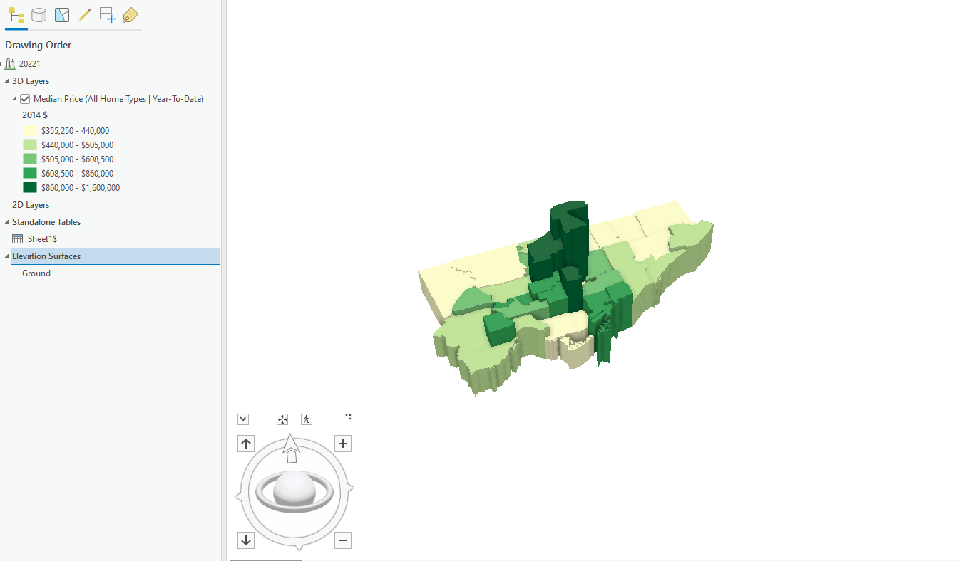
I next needed to display the layers I just created in a 3D environment. From the “Create Tab”, I selected “Create Scene”. A scene viewer page opened and the virtual 3D globe which I used to display my layers was generated. Using the “Modify Scene” tab, I added my six layers that I formatted in the map view from my content. As this scene will become the base of the mapping application, it is important that I configured all the desired setting in the scene view, as these settings will not be able to be changed in the application itself. For example, I altered the order of the layers in my legend, chose a basemap, specified the suns position in the sky, and optimized the performance of the scene in scene settings by ensuring the 3D graphics slide bar was set to Performance rather than quality. I then saved the scene and navigated back to “My Content”.

Creating the Web App

In the “Create” tab, I then created an App using the Web Appbuilder. In the following “Create a web app” pop up, I specified 3D and gave the app a title, a tag, and a brief summary.

I then needed to specify to Scene which I wanted to use as the baselayer for my app. I navigated to the Scene I just created through the “Choose web scene” button in the scene setting window. This then projected my 3D MF layers onto the virtual globe into the map. I then navigated to the theme window and chose a graphic theme for my application.

Adding Functionality

Functionality is added to Web Appbuilder applications through widgets. Widgets are tools that can be added to the application. These tools perform a variety of functions. Also, the number of widgets you can incorporate into an app is based on the theme you have selected, so choose wisely. In my application I chose four main widgets, Legend, About, Layer List and 3D Extrusion. The legend widget simply adds a legend to the app which updates depending on the layer being displayed. I configured the About widget to display text introducing the application. The layer List is the widget which enables the toggling between MF layers. Fnally, the 3D widget allows for several different 3D functionalities. I selected the “Area Extrusion” visualization type to extrude the countries based on their Material Footprint per Capita Values. Along with the 3D extrusion, a display bar is added the app which displays the MF values of each nation. By clicking on a nation name in the display bar, the view automatically zooms to that country. Neat!

Finishing Touches

After all the functionality was added to the application, I added a few finishing touches. A proper summary and description were added to the Web App page, and a simple splash widget was added to introduce the application.

Try it out here!

Try the application out here, and thanks for following along!

https://ryerson.maps.arcgis.com/apps/webappviewer3d/index.html?id=b72c5f9cb9194a1abbff695a7b5b275f

Literacy Percentages and Global Prevalence of HIV Rates

by Anwar Abu Ghosh

Geovis Project Assignment @ryersonGeo,

SA8905, Fall 2018

For my geo-visualization project, I have decided to use ArcGIS Online which is a web-based interactive program to visualize the data. The other dataset was extracted from the world health organization was in the format of a comma delimited values (CSV) file which contains the rates and ranks of some countries in the worlds suffering from HIV. Another data set that was used on this project was literacy rates across different countries in the world, which was downloaded as a CSV from United Nations International Children’s Emergency Fund (UNICEF) website.

ArcGIS Online Definition

ArcGIS Online is a cloud-based application that is used to visualize and map data in a dynamic and interactive method. GIS stands for Geographic Information System, and the method this application works is by adding different layers to create different maps and visualize data. It can be used for 2D and 3D mapping, and in this project, I will be using the proportional mapping. It is a great collaborative web-based application with a secure infrastructure to store data, view data, add layers, manipulate data and share maps with others. This web-based application has base maps and data layers integrated into it, therefore many preinstallations may not be required. I will be using the 30-day free trial of ArcGIS Online with limited features and storage.

ArcGIS Desktop

Due to the limited features in the ArcGIS Online free trial, many properties are disabled such as the join feature and so using a different software to join two datasets was required. To be able to create a choropleth map in ArcGIS Online, the data must be provided in a shapefile (SHP) extension format. Therefore, the need to use ArcMap to join a country shapefile to the literacy rates CSV was needed. The layer was first added by right clicking ‘Layers’ in the table of content and browsing to the country shapefile location that was originally downloaded from thematicmapping.org. Then right-click the added layer and selecting ‘Joins and Relates’ then ‘joins’. For the ‘1. Choose the field in this layer that the join will be based on field select the country column in the shapefile. As for the ‘2. Choose the table to join this layer or load the table from disk’ select the literacy CSV file. Meanwhile for the ‘3. Choose the field in the table to base the join on’ which should be referring to the country name column in the literacy data. Allow the join to retain all records and then press okay. The altered country shapefile will have the literacy columns appended to the end of the shapefile. Now that the shapefile is generated some data cleanup such as deleted unnecessary columns may be done before exporting the shapefile. Shapefile exporting is the was ArcGIS saves the new shapefile and this simple step can be done by right clicking the layer and selecting ‘Data’ then ‘Export Data’ to save the updated shapefile to the desired location. Note to have the shapefile ready for ArcGIS online; the shapefile should be saved in its own folder as multiple files will automatically be generated when creating the file and then the folder should be zipped.

ArcGIS Online Application

Adding the first layer

The first layer in this map will be the literacy data. Start by successfully logging in to ArcGIS Online and selecting the map option in the top bar. Then browse to the map option, click the ‘Add’ option and select the ‘Add Layer from File’. Then browse to the zipped file that was created from the previous step in ArcMap. To create the choropleth map, the percentage column is to be selected as ‘Shows an attribute to show’ and then counts and amounts (Color). Selecting blue from the symbols settings then ‘fill’, this step is done to represent the literacy data where the light shade indicates a low literacy rate and a dark blue indicates a high literacy rate in the country.

Adding Second Layer

Selecting from the toolbar ‘Add layer by file’ from the add setting. Browse to the csv file stored on the computer. Many options will appear on the way the file is to be imported. Using the located feature by selecting ‘by World’ from the drill down option. Match the country column in the HIV data to the country from the preexisting data in ArcGIS Online. The data will then be imported to the application in point form. Create a proportion map by using the proper setting of selecting the proportion based on HIV rates. The color used in displaying the data points is red since the red ribbon is an awareness symbol of HIV/AIDS.

Since many colors and shades are being used in this interactive map a simple light grey canvas was used as a basemap to make the colors and symbols more visible to the reader. As for the legend, it can be found on the left-hand side of the application right under the toolbar. The legend consists of two components the proportionate layer for the HIV/AIDS data where the symbol refers to the percentage of HIV/AIDS rates. The other component refers to the literacy rates where the shade of blue refers to the rate of literacy rate in a country.

Feel free to take a look at the map through this link https://arcg.is/1uPu14

References

http://thematicmapping.org/downloads/world_borders.phphttps://data.unicef.org/topic/education/literacy/

http://apps.who.int/gho/data/node.main.617?lang=en