Mapping Toronto’s Post-War Urban Sprawl & Infill Growth (1945-2021)

A Geovizualization Project by Mandeep Rainal.

SA8905 – Master of Spatial Analysis, Toronto Metropolitan University.

For this project, I explore how Toronto has grown and intensified over time, by creating a 3D animated geovisualization using Kepler.gl. I will be using 3D building massing data from the City of Toronto and construction period information from the 2021 Census data (CHASS).

Instead of showing a static before and after map, I decided to build a 3D animated geovizualization that reveals how the city “fills in” over time showing the early suburban expansion, mid-era infill, and rapid post-2000 intensification.

To do this, I combined the following:

The result is a dynamic sequence showing how Toronto physically grew upward and outward.

BACKGROUND

Toronto is Canada’s largest and fastest growing city. Understanding where and when the built environment expanded helps explain patterns of suburbanization, identify older and newer development areas and see infill and intensification. This also helps contextualize shifts in density and planning priorities for future development.

Although building-level construction years are not publicly available, the City of Toronto provides detailed 3D massing geometry, and Statistics Canada provides construction periods at the census tract level for private dwellings.

By combining these sources into a single animated geovizualization, we can vizualize Toronto’s physical growth pattern over 75 years.

DATA

• City of Toronto – 3D Building Massing (Polygon Data)
  1. Height attributes (average height)
  2. Building Footprints
  3. Used for 3D extrusions

• City of Toronto – Muncipal Boundary (Polygon Data)
  1. Used to isolate from the Census metropolitan area to the Toronto city core.

• 2021 Census Tract Boundary

• CHASS (2021 Census) – Construction Periods for Dwellings
  1. Total dwellings
  2. 1960 and before
  3. 1961-1980
  4. 1981-1990
  5. 1991-2010
  6. 2011-2015
  7. 2016-2021
  8. Used to assign Age classes and a generalized “BuiltYear” for each building.

METHODOLOGY

Step 1: Cleaning and Preparing the Data in ArcGIS Pro

• I first imported the collected data into ArcGIS. I clipped the census tract layers to the City of Toronto boundary to get census tracts for Toronto only.
• Next, I joined the census tract polygon layer we created to the construction period data that was imported. This gives us census tracts with construction period counts.
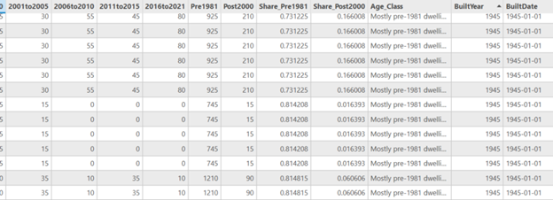
• Because Toronto does not have building-year data, I assigned construction era categories from the census as proxies for building age, and created an age classification system using proportions. Adding periods and dividing / total dwellings to get proportions, and assigned them into three classes:
  • Mostly Pre-1981 dwellings
  • Mixed-era dwellings
  • Mostly 2000+dwellings
• Next, I needed a numeric date field for Kepler to activate the time field. I assigned a representative year to each tract using the Age classes.
  • if age = Mostly Pre-1981 dwellings = 1945
  • if age = Mixed-era dwellings = 1990
  • if age = Mostly 2000+dwellings = 2010
• And to make the built year Kepler-compatible a new date field was created to format as 1945-01-01.
• The data was then exported as GeoJSON files to import into Kepler.gl. The built year data was also exported as a CSV because Kepler doesn’t pick up on the time field in geoJSON easily.

Stage 2: Visualizing the Growth in Kepler

• Once the layers are loaded into Kepler the tool allows you manipulate and vizualize different attributes quickly.
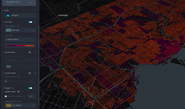
• First the 3D Massing GeoJSON was set to show height extrusion based on the average height field. The colour of the layer was muted and set to be based on the age classes and dwelling eras of the buildings.
• Second layer, was a point layer also based on the age-classes. This would fill in the 3D massings as the time slider progressed, and was based on brighter colours.
• The Built Date CSV was added as a time-based filter for the build date field.

The final visualization was screen recorded and shows an animation of Toronto being built from 1945 to 2021.

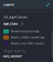
• Teal = Mixed-era dwellings
• Amber = Mostly 2000+ dwellings
• Dark purple = Mostly Pre-1981 dwellings

RESULTS

The animation reveals key patterns on development in the city.

• Pre-1981 areas dominate older neighbourhoods, the purple shaded areas show Old Toronto, Riverdale, Highpark, North York.
• Mixed-era dwellings appear in more transitional suburbs, filling in teal, and showing subdividisions with infill.
• Mostly 2000+ dwellings are filling in amber and highlight the rapid intensification in areas like downtown with high-rise booms, North York centre, Scarborough Town Centre.

The animation shows suburban sprawl expanding outward, before the vertical intensification era begins around the year 2000.

Because Kepler.gl cannot export 3D time-slider animations as standalone HTML files, I captured the final visualization using Microsoft Windows screen recording instead.

LIMITATIONS

This visualization used census tract–level construction-period data as a proxy for building age, which means the timing of development is generalized rather than precise. I had to collapse the CHASS construction ranges into age classes because the census periods span multiple decades and cannot be animated in Kepler.gl’s time slider, which only accepts a single built-year value per feature. Because all buildings within a tract inherit the same age class, fine-grained variation is lost and the results are affected by aggregation. Census construction categories are broad, and assigning a single representative “built year” further simplifies patterns. The Kepler animation therefore illustrates symbolic patterns of sprawl, infill, and intensification, not exact chronological construction patterns.

CONCLUSION

This project demonstrates how multiple datasets can be combined to produce a compelling 3D time-based visualization of a city’s growth. By integrating ArcGIS Pro preprocessing with Kepler’s dynamic visualization tools, I was able to:

• Simplify census construction-era data
• Generate meaningful urban age classes
• Create temporal building representations
• Visualize 75+ years of urban development in a single interactive tool

Kepler’s time slider adds an intuitive, animated story of how Toronto grew, revealing patterns of change that static maps cannot communicate.